
Executive Summary
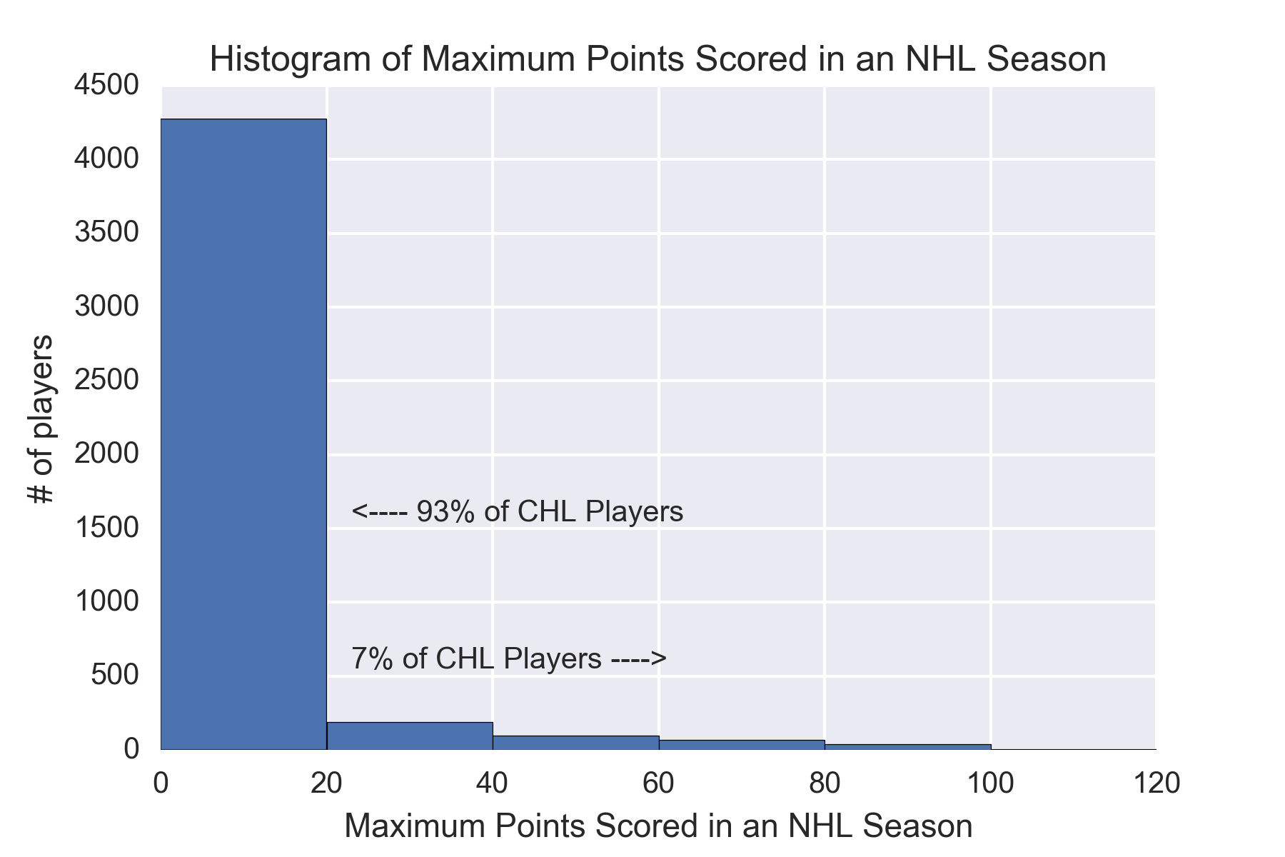
A significant part of any sports teams’ success is effective player drafting and acquisition. The NHL is no different in this regard and has been ramping up the use of data analytics to help improve efficiency in these areas. In this project, I examined players from the Canadian Hockey League (CHL) (a composite of the Ontario Hockey League (OHL), Western Hockey League (WHL), and Quebec Major Junior Hockey League (QMJHL)) and built a classifier to predict whether or not a player would make it to the NHL and record at the minimum a 20 point season. There are a number of different ways to measure NHL success, Jonathan Willis makes the case that 200-games played in the NHL is a strong cut-off as to whether a prospect has “made it” in the NHL[5]. I wanted to look at offensive capabilities, so I decided upon the 20 point mark which only 38% (612/1591) of players reached this mark from NHL seasons 2011-2016 [6]. I found that only about 7% of players from our training CHL dataset ever actually record 20+ point season in the NHL, and that some of the best indicators for this criteria of success are age, assists per game, power play assists per game and power play goals per game. Unsurprisingly, I found that while it was very easy to predict the players who were unlikely to make it, the players who did reach the 20+ point mark had a very wide range of statistical production at the CHL level, making it very hard to predict the “winners” from the cohort.
There are some other interesting analyses on player prospecting. Most similarly, the proposed Prospect Cohort Success (PCS) model from Josh Weissbock, looks at evaluating CHL players by comparing them to existing NHL players and using that score to predict the probability that the player will reach the NHL[2]. Another useful tool and popular approach for evaluating prospects success is to project their expected scoring capabilities were they to jump to the NHL[8] or to determine how many goals is worth in one league translates to another[9]. Below I will walk through the data used in this process, the evaluation of models and the information you can glean from this study.
Data Collection
In order to build my CHL classifier model, I had to pull historical data from the CHL leagues. I was able to pull data directly from the three leagues websites ohl.ca[10], ontariohockeyleague.com[11] and theqmjhl.ca[12]. The websites had data back to the 1997-98 seasons, and as such that was the beginning of my data for modeling. I looked for some general baseline on peak performance in the NHL to see where an appropriate cut-off may be for the upper end. One estimation suggest that peak per-game point performance peaks at ages 24-26 [7]. Using this guideline, I used the 2004-05 season as the cutoff on the upper end of the data. With the youngest of these players being ~29 years of age at the time we pulled their NHL performance, I worked under the assumption that the players from the 98-05 seasons, had already reached their full potential.
I pulled NHL data from hockey-reference.com[13] from 97-98 through 2015-16 NHL seasons. Once I had the CHL datasets and NHL datasets loaded, I put the NHL dataset into a pivot table, with the player as the index and the aggregating fuction as a max function, so that I had a list of NHL players with their highest full season point total from 98-16. From here I matched up the NHL max points season dataset with the CHL dataset on player’s names to give us our target variable for the analysis. There were some manual connections that were necessary to ensure that players names from the hockey-reference database matched the CHL databases (e.g Pierre-Alexandre Parenteau & P.A. Parenteau). There were also instances where it was necessary to distinguish between two players with the same name. From here I had a master CHL database with our target variable attached to the dataframe.
Data Import
Once collected and combined, the dataset was imported to work on the modeling process.
chl = pd.read_csv('../Combined CHL Data/chl_98_16_pts_bin.csv')
# reorder by season and reset index
chl = chl.sort_values(by='season_start_date', ascending=False).reset_index()
Data Preprocessing
At this stage in the process I had to select what statistics I wanted to work with. A number of statistics such as shots and shot percentage were not tracked during the 98-05 seasons and were not consistent across all three leagues. What I was left with was the below list.
keep_list = ['full_name', 'birthdate', 'rookie', 'points_per_game',
             'position', 'penalty_minutes_per_game', 'games_played',
             'weight', 'season', 'team_id', 'points', 'assists', 'goals',
             'power_play_assists', 'season_start_date', 'power_play_goals',
             'short_handed_assists', 'short_handed_goals', 'unassisted_goals',
             'league', 'max_pt_season_bin', 'unassisted_goals', 'points',
             'overtime_goals', 'empty_net_goals']

X = chl[keep_list]
Prior to starting any of our models and analysis, I wanted to look at a base model and get a sense for what the success rate was for the players from the CHL making it to the 20 point mark in the NHL. This will be extremely valuable for later evaluating how well our model does. If I can’t beat the values here our model is not much better than selecting all players to not make the 20 point mark in the NHL.
# watermark for a base model w/ using player data from 98-05
b = pd.pivot_table(X_fin, index='full_name',
                   aggfunc=np.mean).max_pt_season_bin.value_counts()
(b / sum(b)) * 100

0.0     92.999110
20.0     3.619104
40.0     1.720558
60.0     1.661228
Name: max_pt_season_bin, dtype: float64
Datetime Conversion
I made sure the appropriate categories were converted objects to datetime so that I could calculate season start date, birthdate, and season start age for each player. Using birthdate instead of year will give a much greater granularity on players performance at a given age.
# convert birthdate and season start date to datetime
X.loc[:, 'birthdate'] = pd.to_datetime(X.loc[:, 'birthdate'])
X.loc[:, 'season_start_date'] = pd.to_datetime(X.loc[:, 'season_start_date'])
def age_diff(season_start, birthdate):
    # returns the difference between season start date and birthday
    return (season_start - birthdate)


# calculates the season start age age
X.loc[:, 'season_start_age'] = age_diff(
    X.loc[:, 'season_start_date'], X.loc[:, 'birthdate'])

# convert season start_age to years
X.loc[:, 'season_start_age'] = [
    (i / np.timedelta64(1, 'D')) / 365 for i in X.season_start_age]
Generating Per Game Stats
While pure point production can sometimes be valuable, I wanted to specifically look at per-game production to include players who may have bloomed late or had seasons cut short due to injuries.
def per_game_stats(games_played, stat_column):
    # returns the difference between season start date and birthday
    return (stat_column / games_played)


X.loc[:, 'apg'] = per_game_stats(X.loc[:, 'games_played'], X.loc[:, 'assists'])
X.loc[:, 'gpg'] = per_game_stats(X.loc[:, 'games_played'], X.loc[:, 'goals'])
X.loc[:, 'sh_gpg'] = per_game_stats(
    X.loc[:, 'games_played'], X.loc[:, 'short_handed_goals'])
X.loc[:, 'sh_apg'] = per_game_stats(
    X.loc[:, 'games_played'], X.loc[:, 'short_handed_assists'])
X.loc[:, 'pp_apg'] = per_game_stats(
    X.loc[:, 'games_played'], X.loc[:, 'power_play_assists'])
X.loc[:, 'pp_gpg'] = per_game_stats(
    X.loc[:, 'games_played'], X.loc[:, 'power_play_goals'])

# create  per game values squared to try and isolate top performers better
X.loc[:, 'apg2'] = X.loc[:, 'apg'].apply(lambda x: pow(x, 2))
X.loc[:, 'gpg2'] = X.loc[:, 'gpg'].apply(lambda x: pow(x, 2))
X.loc[:, 'pp_apg2'] = X.loc[:, 'pp_apg'].apply(lambda x: pow(x, 2))
X.loc[:, 'pp_gpg2'] = X.loc[:, 'pp_gpg'].apply(lambda x: pow(x, 2))
Given that I was looking at a per game basis for point production, I removed a few of the features that were used to generate the per game stats.
drop_list = ['season_start_date', 'short_handed_goals', 'short_handed_assists',
             'power_play_assists', 'power_play_goals', 'unassisted_goals',
             'draft_day']
X = X.drop(drop_list, axis=1, errors='ignore')
Dealing with Missing Values and Categorical Data
# replace NaN weights with the mean value of weights
X.loc[:, 'weight'] = X.loc[:, 'weight'].fillna(
    value=round(X.loc[:, 'weight'].mean(), 2))
pos_dum = pd.get_dummies(X.position)
league_dum = pd.get_dummies(X.league)
Data cleaning
Once I had a DataFrame with the features I desired, I looked into filtering the DataFrame further based on some assumptions that I wanted to make about the data. First off, I removed all goalies from the dataset as goalies do not score very many points, and whether or not they do is really not a point of interest for me at this time. I also removed a few data points where the players start ages were well over 22. Within the CHL database there were a few birthdays that were not known and thus provided a birth year of -1, which severely skewed the models I built. Another option would have been to impute the mean value, but given the small amount of players this affected, I removed them all toegether.
df_final = df_final[(df_final.G != 1)]  # filter out goalies
# filters out errors in birthdate
df_final = df_final[df_final.season_start_age < 22]
# drop the unnecessary columns
df_final = df_final.drop(['G'], axis=1, errors='ignore')
df_final = df_final.reset_index().drop(
    ['level_0', 'index'], axis=1, errors='ignore')
y = df_final[['max_pt_season_bin', 'season', 'full_name']]
I renamed some of the columns and shortened them so that they were easier to reference and visualize in the heatmap.
df_final = df_final.rename(columns={'penalty_minutes_per_game': 'pim_pg',
                                    'max_pt_season_bin': 'max_pt_season',
                                    'empty_net_goals': 'en_goals',
                                    'overtime_goals': 'ot_goals'})
sns.heatmap(df_final.corr())
plt.xticks(rotation=90)
plt.tight_layout()
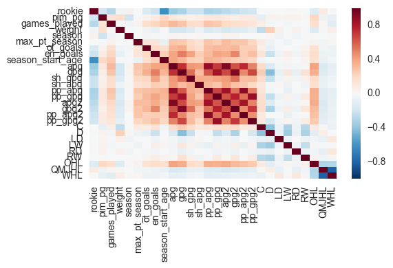
Taking a look at the heatmap you can see that there are a number of features that are highly correlated with eachother. Since I was dealing with a number of statistics that are either subsets of eachother (short handed assists per game and assists per game) or derivatives of eachother (asissts per game and assists per game squared), it makes intuitive sense that there would be these correlations.

Taking a look at the target variable max_pt_season, it’s also evident that there is some correlation between point production statistics and our desired outcome of a 20+ point NHL season.
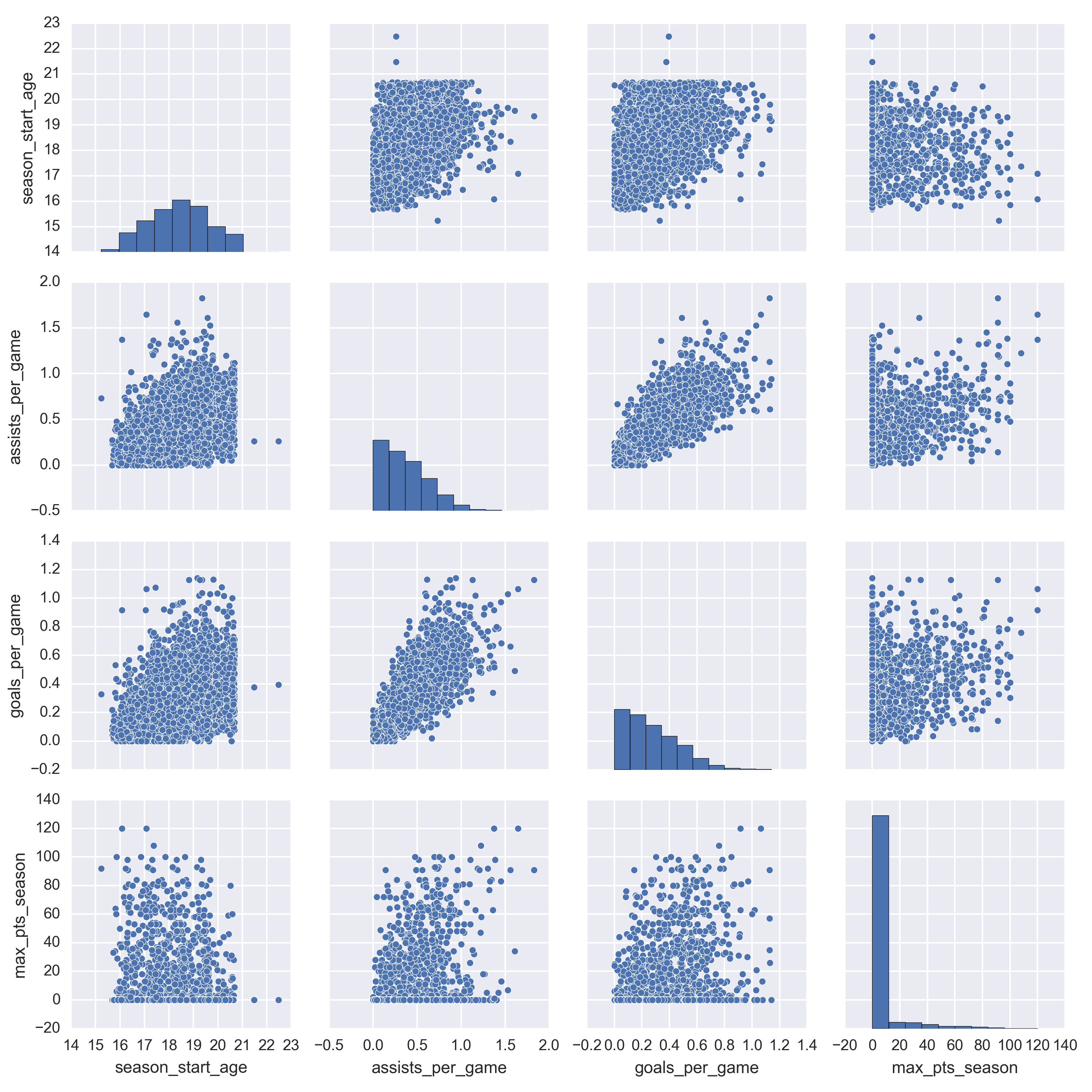
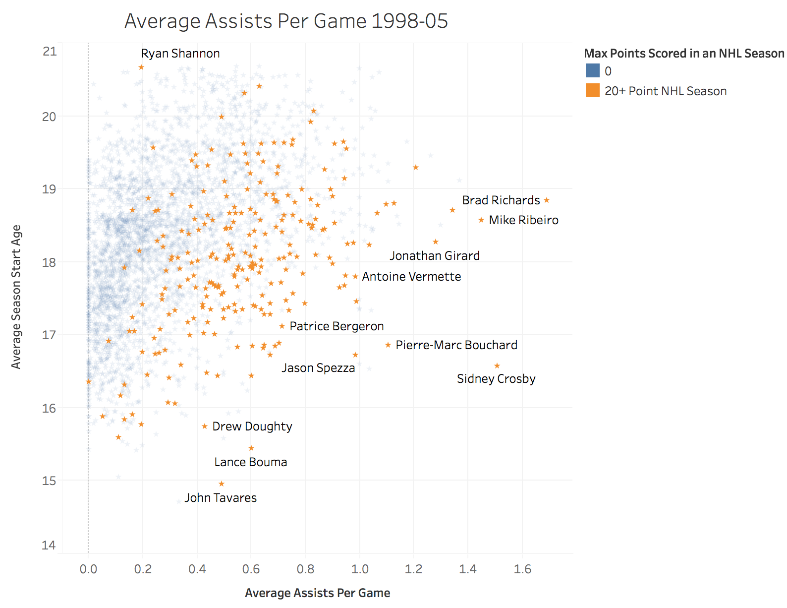
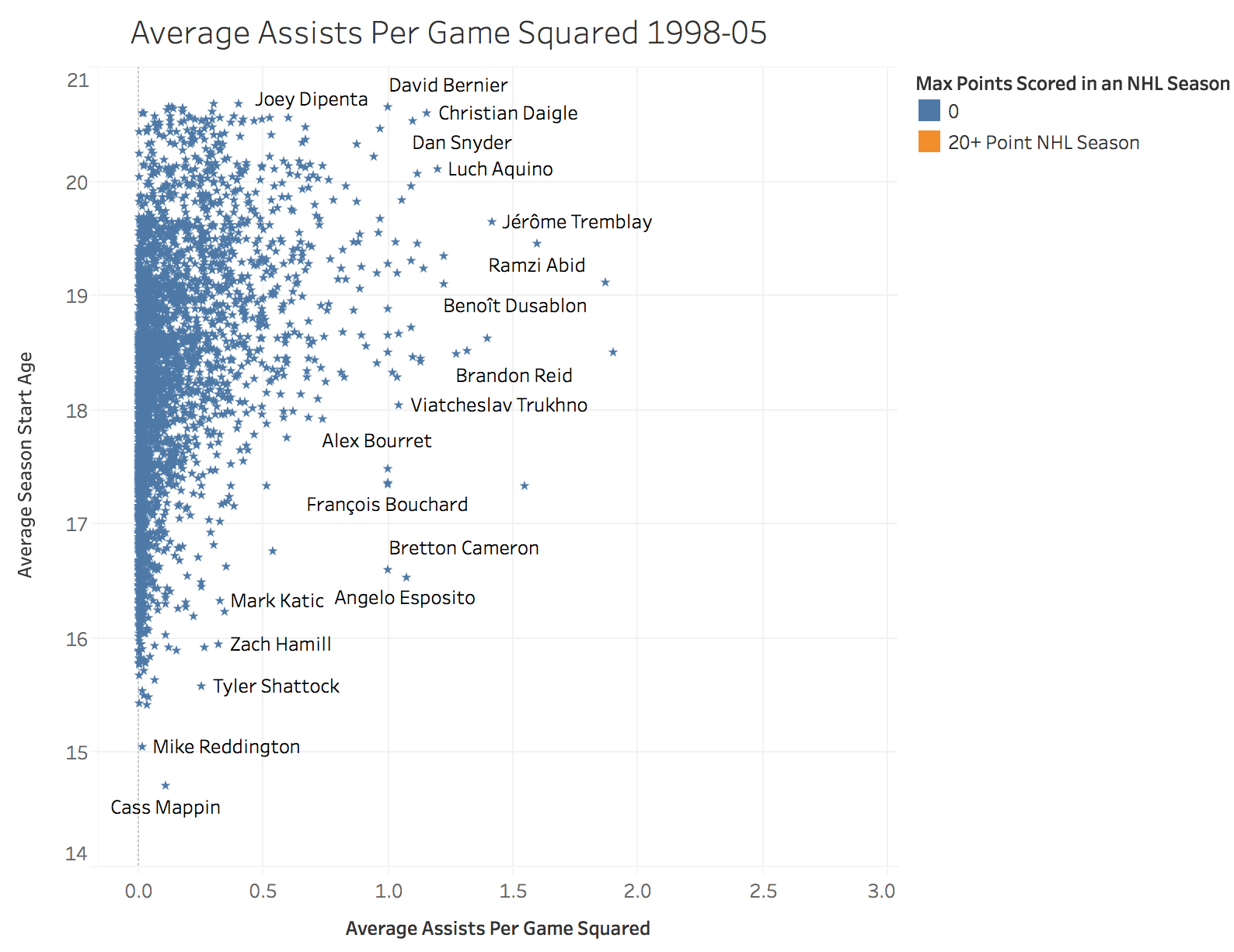
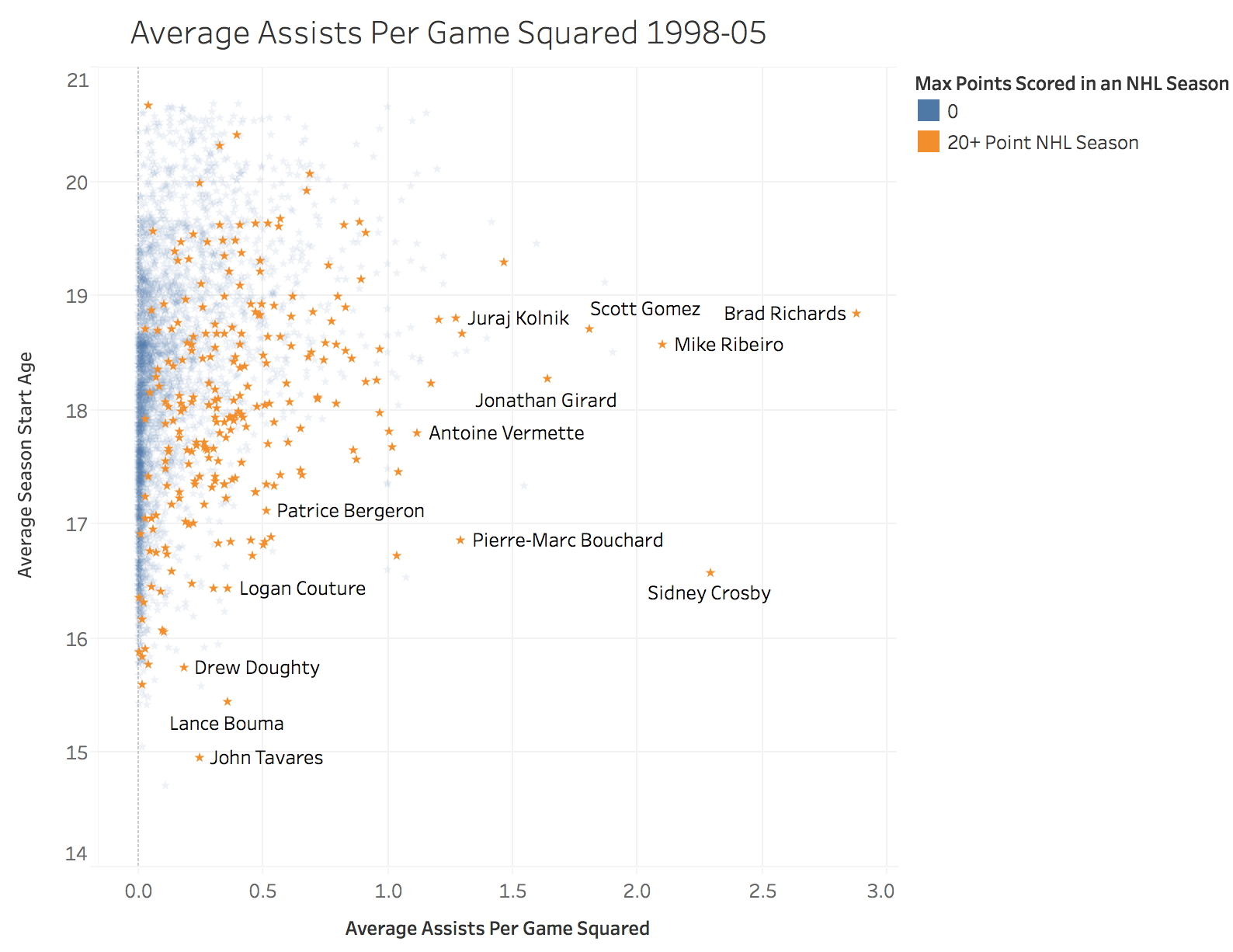
In the pairplot I produced, it is evident that there is quite a bit of noise. There is a large subset of players with very high assists per game and goals per game production at a very young age that never even make it to the NHL. There is a slight up and to the right trend for the assists per game and goals per game and a slight up and to the left for the season start age plots.
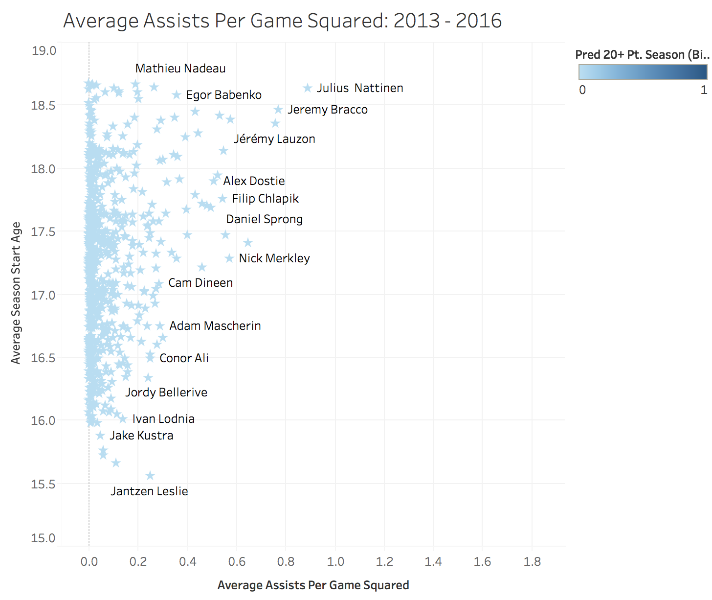
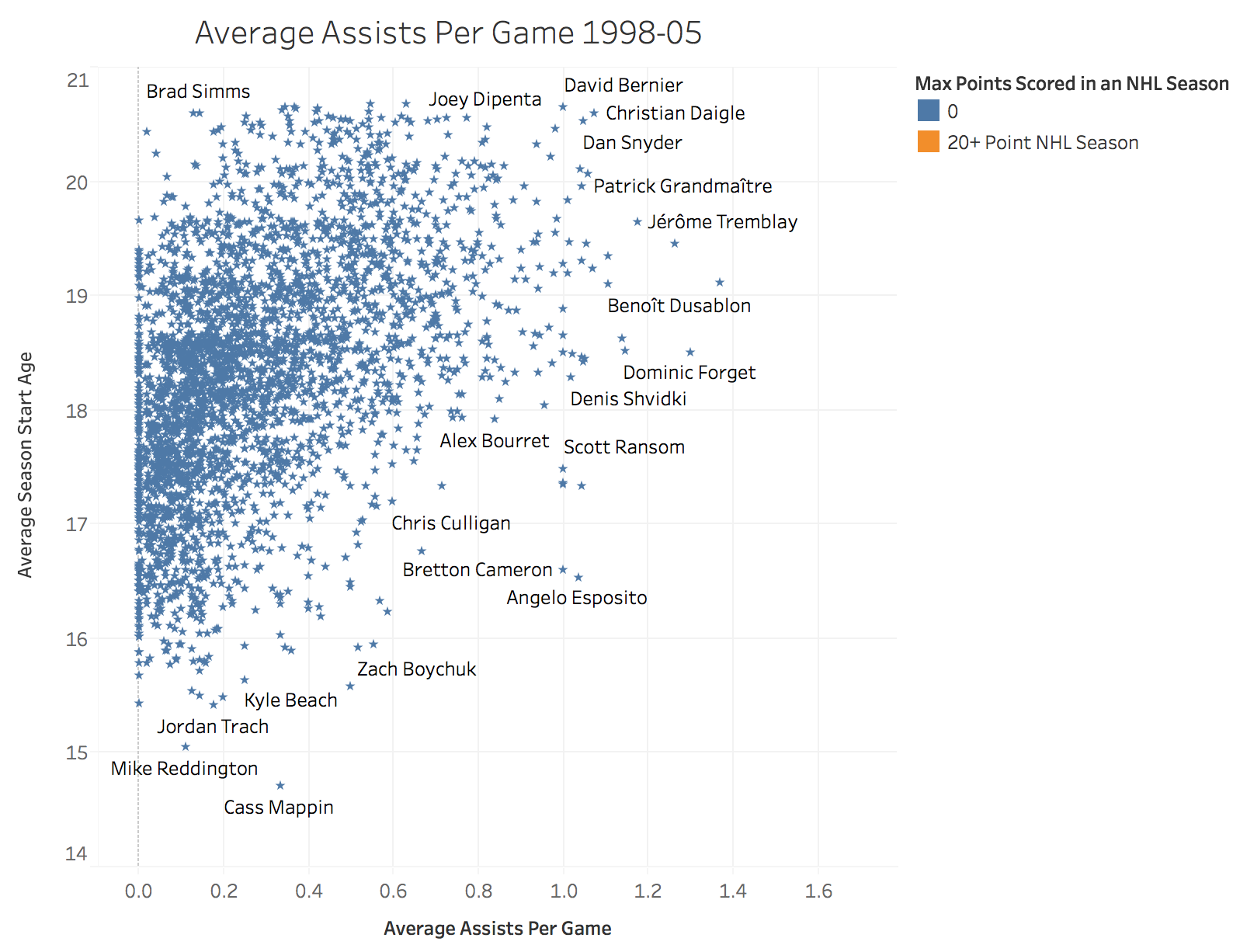 In addition when looking at the assists per game by season start age scatter plot we can see that there’s no clear delineation between features. A simple logistic regression or SVM model will not suffice to differentiate between the players who make it and those who don’t. I used this exploratory data analysis to help guide my decision making as we moved through the modeling phase.
While I pulled all CHL data from 98-16, I had to decide upon a cutoff on the upper end of our data. The reason for this as described in the introduction is because I needed to make a distinction about a point in time that I can reasonably assume a players production has “settled”. In other words, I am making the assumption that players from the 2004-05 season (which are at a minimum 29 years of age as of the 2015-2016 season) will not change whether or not they meet my production criteria.
Filter by the cutoff season
# split by season since the newer seasons will be harder to predict

season_cutoff = 6  # not inclusive so it will cutoff at 2005

X_fin = df_final[(df_final['season'] < season_cutoff)
                 | (df_final['season'] > 90)]
y = y[(y['season'] < season_cutoff) | (y['season'] > 90)]


# will not be able to verify but for fun
draft_eligible_test = df_final[(df_final['season'] > 12)
                          & (df_final['season'] < 90)]
draft_eligible_17 = draft_eligible[
    (draft_eligible.birthdate > datetime(1997, 1, 1))
    & (draft_eligible.birthdate < datetime(1999, 9, 15))]
I used pivot tables to average the metrics in order to get a players full body of work as well as to account for the fact that we were looking at a few years of production.
X_piv = pd.pivot_table(X_fin, index='full_name', aggfunc=np.mean).drop(
    ['season', 'max_pt_season_bin'], axis=1)
y_piv = pd.pivot_table(y, index='full_name',
                       aggfunc=np.mean).drop(['season'], axis=1)

# for final analysis
draft_eligible_17 = pd.pivot_table(
    draft_eligible_17, index='full_name', aggfunc=np.mean).drop([
        'season', 'max_pt_season_bin'], axis=1, errors='ignore')
# reset the index and drop the full name so we can put this through
# the train test split
X_piv_r = X_piv.reset_index().drop('full_name', axis=1)
y_piv_r = y_piv.reset_index().drop('full_name', axis=1)

# for final analysis
final_test = draft_eligible_17.reset_index()
draft_eligible_17_final = draft_eligible_17.reset_index().drop('full_name', axis=1)
len(X_piv_r), len(y_piv_r), len(draft_eligible_17_final)
Splitting the Training and Testing Data
X_train, X_test, y_train, y_test = train_test_split(
    X_piv_r, y_piv_r, test_size=0.25, random_state=42)

# convert to binary classifier for y_train & y_test
y_train_binary = y_train.max_pt_season_bin.apply(convert_to_binary)
y_test_binary = y_test.max_pt_season_bin.apply(convert_to_binary)
Model Selection
Now that I had the data into my training and testing splits, I started putting them into a few classification models. I started with exploring a basic logistic regression model. While this model performed very well on predicting the players who did not make it to the point threshold, it performed very poorly on predicting the players who would exceed the point threshold. With a precision score of 0.16 and an f1-score of 0.26 on the predicted variable, it was evident I would have to do some additional feature engineering, parameter searching and modeling.
All in all I tested 6 models & methods (Decision Trees, Random Forest, Logistic Regression, SVM, AdaBoost, KNN). The code for those models and the results are shown below.
Logistic Regression
X_train = ss.fit_transform(X_train)
X_test = ss.fit_transform(X_test)

logit = LogisticRegression(penalty='l2', C=0.001, class_weight='balanced')

model_a = logit.fit(X_train, np.ravel(y_train_binary))
y_pred = model_a.predict(X_test)


confmat_logit = confusion_matrix(y_true=y_test_binary, y_pred=y_pred)
confusion_matrix_logit = pd.DataFrame(confmat_logit,
                                      index=['Actual MPS < 20',
                                             'Actual MPS > 20'],
                                      columns=['Predicted MPS < 20',
                                               'Predicted MPS > 20'])
			 Logistic Regression Performance

             precision    recall  f1-score   support

          0       0.99      0.72      0.83       796
          1       0.16      0.87      0.26        47

avg / total       0.94      0.73      0.80       843


                 Predicted MPS < 20  Predicted MPS > 20
Actual MPS < 20                 573                 223
Actual MPS > 20                   6                  41
Logistic Regression (Grid Search)
# pipeline for GS
pipe_lr = Pipeline([('scl', StandardScaler()),
                    ('clf', LogisticRegression(random_state=1))])

param_range = [0.0001, 0.001, 0.01, 0.1, 1.0, 10.0, 100.0, 1000.0]

param_grid = {'clf__C': param_range,
              'clf__penalty': ['l1', 'l2']}

gs = GridSearchCV(estimator=pipe_lr,
                  param_grid=param_grid,
                  scoring='accuracy',
                  cv=10,
                  n_jobs=-1)
gs = gs.fit(X_train, np.ravel(y_train_binary))
print(gs.best_score_)
print(gs.best_params_)
0.928006329114
{'clf__penalty': 'l1', 'clf__C': 0.1}
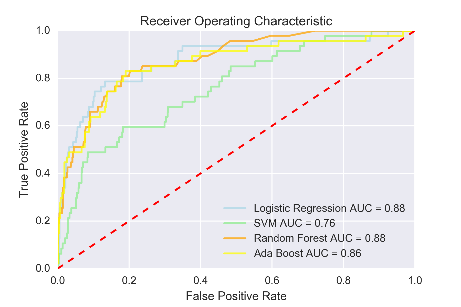
Through this process I grid searched my models hyperparameters. I’ve shown the Logistic Regression grid search and excluded the others for simplicity. When looking at the results you can see that across a number scoring metrics, AUC, Accuracy, F1, F1_micro, F1_macro, the results were poor and noisy at predicting the players to have success in the NHL.
Support Vector Machines (SVM)
from sklearn.svm import SVC

X_train = ss.fit_transform(X_train)
X_test = ss.fit_transform(X_test)

svm = SVC(probability=True, C=10, kernel='rbf', degree=3)

model_svm = svm.fit(X_train, np.ravel(y_train_binary))
y_pred_svm = model_svm.predict(X_test)

confmat_svm = confusion_matrix(y_true=y_test_binary, y_pred=y_pred_svm)
			 SVM Performance

             precision    recall  f1-score   support

          0       0.96      0.97      0.97       796
          1       0.42      0.32      0.36        47

avg / total       0.93      0.94      0.93       843


                 Predicted MPS < 20  Predicted MPS > 20
Actual MPS < 20                 775                  21
Actual MPS > 20                  32                  15
Random Forest Classifier
# grid search for Random Forest classifier
rfc = RandomForestClassifier()

parameters = [{"n_estimators": [250, 500, 1000],
              "max_depth": [3, 5, 7, 9, 11, None],
              "max_features": np.arange(3,27),
              "bootstrap": [True, False],
              "criterion": ["gini", "entropy"]}]

# Returns the best configuration for a model
def best_config(model, parameters, train_instances, judgements):
    clf = GridSearchCV(model, parameters, cv=5,
                       scoring="f1_macro", verbose=5, n_jobs=4)
    clf.fit(train_instances, judgements)
    best_estimator = clf.best_estimator_

    return [str(clf.best_params_), clf.best_score_,
            best_estimator]


best_config(rfc, parameters, X_train, np.ravel(y_train_binary))
Ada Boost
tree = DecisionTreeClassifier(criterion='entropy',
                              max_depth=8,
                              random_state=0)

ada = AdaBoostClassifier(base_estimator=tree,
                         n_estimators=1000,
                         learning_rate=1.0,
                         random_state=0)
tree = tree.fit(X_train, np.ravel(y_train_binary))
y_train_pred = tree.predict(X_train)
y_test_pred = tree.predict(X_test)

tree_train = f1_score(y_train_binary, y_train_pred)
tree_test = f1_score(y_test_binary, y_test_pred)
print('Decision tree train/test accuracies %.3f/%.3f'
      % (tree_train, tree_test))

ada = ada.fit(X_train, np.ravel(y_train_binary))
y_train_pred = ada.predict(X_train)
y_test_ada = ada.predict(X_test)

ada_train = f1_score(np.ravel(y_train_binary), y_train_pred)
ada_test = f1_score(np.ravel(y_test_binary), y_test_ada)

print('AdaBoost train/test accuracies %.3f/%.3f'
      % (ada_train, ada_test))
Decision tree train/test accuracies 0.765/0.310
AdaBoost train/test accuracies 1.000/0.300
confmat_tree = confusion_matrix(y_true=y_test_binary, y_pred=y_test_tree)
confmat_ada = confusion_matrix(y_true=y_test_binary, y_pred=y_test_ada)
			 Decision Tree Performance
             precision    recall  f1-score   support

          0       0.96      0.97      0.96       796
          1       0.33      0.26      0.29        47

avg / total       0.92      0.93      0.93       843

                 Predicted MPS < 20  Predicted MPS > 20
Actual MPS < 20                 772                  24
Actual MPS > 20                  35                  12


			 Ada Boost Performance
             precision    recall  f1-score   support

          0       0.95      0.99      0.97       796
          1       0.69      0.19      0.30        47

avg / total       0.94      0.95      0.94       843

                 Predicted MPS < 20  Predicted MPS > 20
Actual MPS < 20                 792                   4
Actual MPS > 20                  38                   9
After running through all these results, I chose the Random Forests model, which generated the best f1-score. While ada-boost method had much better precision, it was at the expense of recall. The random forests method I chose with the grid searched parameters are below.
Best Grid Searched Model
# define the model parameters
rfr_gs = RandomForestClassifier(max_features=10, n_estimators=500, bootstrap=False,
                                     criterion='entropy', max_depth=None, n_jobs=4)

# train the model
rfr_gs_model = rfr_gs.fit(X_train, np.ravel(y_train_binary))

# predict the values on the test set
y_pred_rfr = rfr_gs_model.predict(X_test)
# construct the confusion matrix
confmat_rfc = confusion_matrix(y_true=y_test_binary, y_pred=y_pred_rfr)
	 Random Forest Classifier Performance
	 *MPS - Max points scored in an NHL season*

                 Predicted MPS < 20  Predicted MPS > 20
Actual MPS < 20                 784                  12
Actual MPS > 20                  33                  14


             precision    recall  f1-score   support

   MPS < 20       0.96      0.98      0.97       796
   MPS > 20       0.54      0.30      0.38        47

avg / total       0.94      0.95      0.94       843
feature_importance = pd.DataFrame(
    rfr_gs_model.feature_importances_, index=X_piv_r.columns).sort_values(by=0, ascending=True)
feature_importance = feature_importance.rename(
    columns={0: 'Relative Importance'})
feature_importance.plot(kind='barh')
plt.title('Feature Importance')
plt.tight_layout()
plt.show()

A Look at the Top Performing Feature
Results
In our final model, the most important features were season start age, assists per game squared and power-play asissts per game squared. The ADA boost method also provided fairly good results with 69% precision, however it provided better precision at the cost of recall and the overall f1 score versus the Random Forests Classifier. The results hammer home a few important points. The first is that high level production at the Major Junior level still does not guarantee a baseline level of success at the NHL. Even some of the best performers at a young age sometimes fail to make even a modest impact at the next level. I will speculate that much of this has to do with the fact that there is so much physical development that goes on in between the age 15-18 seasons and a player in their point scoring prime in the NHL at age 24-26.
Additionally, I think this study lends further creedence to the idea that there should be an increased look at advanced analytics being used in the Junior league levels. The NHL has started to embrace this with a few teams hiring members from the hockey analytics community, most recently & notably WAR ON ICE co-founder Sam Ventura was hired to the Pittsburgh Penguins to head their analytics staff in 2015[14]. There are a few people who are doing some interesting work to pull additional statistics out of these games beyond the popular corsi and fenwick. For instance, Ryan Stimson’s Expected Primary Points would be a great stat to add into this CHL model[15]. Unfortunately since much of this data was not tracked historically there will always be incomplete player profiles when looking at old CHL data.

Examining Classes from 13-16 Seasons using the Random Forests Classifier
draft_17_preds = rfr_gs_model.predict(draft_eligible_17_final)
draft_eligible_predictions = pd.concat(
    [final_test, pd.DataFrame(draft_17_preds)], axis=1)
draft_eligible_predictions[['full_name', 'season_start_age',
                            'apg2', 'gpg2', 0]].sort_values(0, ascending=False)
draft_eligible_predictions.head()
| full_name | C | D | LD | LW | OHL | QMJHL | RD | RW | WHL | ... | pp_apg | pp_apg2 | pp_gpg | pp_gpg2 | rookie | season_start_age | sh_apg | sh_gpg | weight | 0 | |
|---|---|---|---|---|---|---|---|---|---|---|---|---|---|---|---|---|---|---|---|---|---|
| 0 | Aaron Boyd | 0.0 | 0.0 | 0.0 | 1.0 | 0.0 | 1.0 | 0.0 | 0.0 | 0.0 | ... | 0.000000 | 0.000000 | 0.008197 | 0.000134 | 0.500000 | 17.784932 | 0.000000 | 0.019231 | 190.0 | 0 |
| 1 | Aaron Hyman | 0.0 | 1.0 | 0.0 | 0.0 | 0.0 | 1.0 | 0.0 | 0.0 | 0.0 | ... | 0.000000 | 0.000000 | 0.000000 | 0.000000 | 1.000000 | 17.380822 | 0.000000 | 0.000000 | 215.0 | 0 |
| 2 | Aaron Luchuk | 1.0 | 0.0 | 0.0 | 0.0 | 0.0 | 0.0 | 0.0 | 0.0 | 1.0 | ... | 0.073749 | 0.007366 | 0.022169 | 0.000544 | 0.500000 | 17.919178 | 0.014925 | 0.014816 | 180.0 | 0 |
| 3 | Adam Musil | 1.0 | 0.0 | 0.0 | 0.0 | 0.0 | 1.0 | 0.0 | 0.0 | 0.0 | ... | 0.082323 | 0.007338 | 0.066667 | 0.005038 | 0.333333 | 17.446575 | 0.005051 | 0.010101 | 203.0 | 0 |
| 4 | Adam Berg | 0.0 | 0.0 | 0.0 | 1.0 | 0.0 | 1.0 | 0.0 | 0.0 | 0.0 | ... | 0.000000 | 0.000000 | 0.000000 | 0.000000 | 1.000000 | 18.083562 | 0.000000 | 0.000000 | 200.0 | 0 |
| 5 | Adam Craievich | 0.0 | 0.0 | 0.0 | 0.0 | 0.0 | 0.0 | 0.0 | 1.0 | 1.0 | ... | 0.010278 | 0.000159 | 0.010278 | 0.000159 | 0.333333 | 17.326027 | 0.000000 | 0.000000 | 190.0 | 0 |
689 rows × 28 columns

Once I ran the existing model on the most recent classes of CHL prospects we see some fun results. As of writing this 4 of the 28 players the model has predicted to succeed a 20+ point NHL season have surpassed that mark (Travis Konecney, Connor McDavid, Ivan Proverov and Mitch Marner). Given that the results for all the below players will not be determined for a number of years it will be interesting to see how all of these careers play out. I’m also interested to see how the three undrafted players that were predicted successes pan out (Nolan Patrick, Kailer Yamamoto and Antoine Morand).

- Players highlighted in yellow have already succeeded a 20+ point season in the NHL
- Players highlighted in orange are undrafted (as of February 2017)
- Numbers next to undrafted players are draft rankings (as of February 2017)
References:
- Draft by Numbers: Using Data and Analytics to Improve National Hockey League (NHL) Player Selection Other Sports 1559 © Michael E. Schuckers, Statistical Sports Consulting, LLC
- http://canucksarmy.com/2015/5/26/draft-analytics-unveiling-the-prospect-cohort-success-model
- http://www.theprojectionproject.com/Home/Search
- http://hockeyanalytics.com/2004/12/league-equivalencies/
- http://oilersnation.com/2015/1/23/development-and-the-200-game-mark
- Data pulled from Hockey Reference
- http://www.arcticicehockey.com/2010/1/21/1261318/nhl-points-per-game-peak-age?_ga=1.98974686.1956457380.1427732150
- http://www.behindthenet.ca/projecting_to_nhl.php
- http://hockeyanalytics.com/2004/12/league-equivalencies/
- http://www.ohl.ca
- http://www.ontariohockeyleague.com
- http://www.theqmjhl.ca
- http://www.hockey-reference.com
- http://www.thehockeynews.com/news/article/penguins-hire-war-on-ice-co-creator-want-to-build-analytics-team
- https://hockey-graphs.com/2017/01/19/expected-primary-points-are-a-better-predictor-of-future-scoring-than-shots-points/